LLM Scaling Laws
Training language models is an expensive business and it is important to plan carefully ahead of training. This post will briefly touch studies on scaling laws.
For a given amount of training flops, there is a trade-off between model size and size of dataset. The optimal size for a given amount of compute, is proportional to compute raised to some power α > 1 (The same holds true between FLOPs and dataset size). Different studies have found different α values but there is a wide consensus on the power-law relationship.
Scaling laws tries to answer the following question: Given a compute budget what is the optimal amount of tokens to train a model?
Kaplan scaling laws
First popular study on scaling laws is done by Jared Kaplan of OpenAI [1].
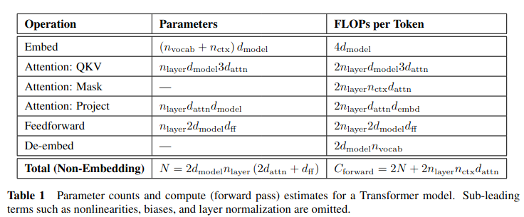
Table 1 shows formula for computing FLOPs per token for forward pass. Since number of parameters of a large language model is significantly greater than context length, context dependent terms is generally omitted. As another approximation, backward pass FLOPs are assumed to be 2 times the forward pass.
Consequently relation between total number of FLOPs C, total tokens D and number of parameters N is given by:
\[C = 6 * N * D\]Kaplan scaling laws assumes a power law relationship between optimal number of parameters and compute and a power law relationship between optimal number of tokens and compute. According to Table 6 of [1] the scaling laws can be expressed as:
\[N \propto C^{0.73}\] \[D \propto C^{0.27}\]These formulations indicate that it is necessary to increase model size and training set size together. However, increase in dataset size is less significant.
Chinchilla scaling laws
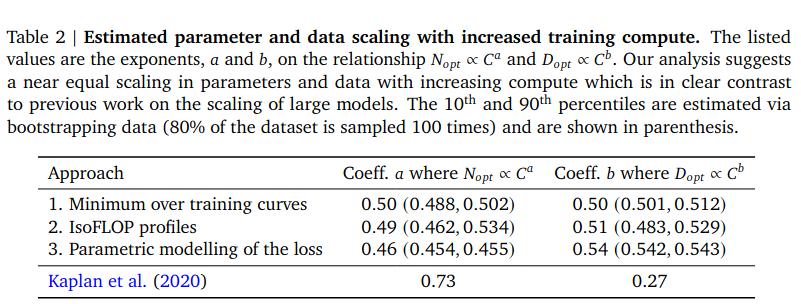
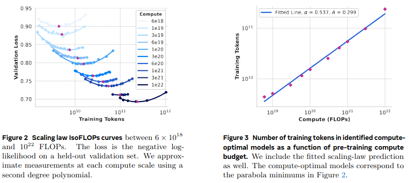
Later in [2] those findings are invalidated. Chinchilla scaling laws assumes similar power-law relationships but claims that dataset size should be increased at the same rate with the model size. They followed 3 different approaches and introduced 3 different scaling relationships. (See Table 2 of [2]).
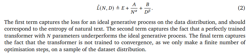
In [2], training loss is modelled as a function of dataset size and model size.
Estimations for the unknown values are given in appendix D.2 of [2].
Using the values it is possible to formulate optimal number of tokens and parameters as in equation 4 of [2].

However, using the estimated parameter values from appendix D.2 of [2], I was unable to recrate results in Table 3 of [2].
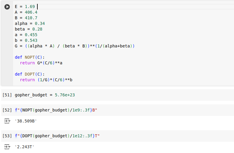
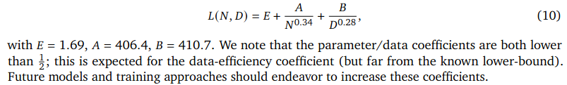
Using the equation 10 with predicted values, I found for a given budget of 5.7e+23 FLOPs, a model with 38B parameters should be trained on 2.2T tokens. But according to Table 3 of [2], model size should have been 67B, dataset size should have been 1.5T. This mismatch is probably due to lack of precision in the given parameter values. In this form these numbers are useless.
Fitting a Linear Line
In [2], Figure A3 shows a linear plot of model training params belonging to all three approaches. Data used for line fitting can be found in Table 3 and Table A3. In Figure A3, it is visible that 3 approaches lead to 3 different lines. Approach 1 and approach 2 resulted in a slightly similar line, while approach 3 produced a significantly different line. The fact that approach 1 and approach 2 outcomes agree to some extent, they can be used to make projections about determining the number of tokens given a model size. It would not be a reliable estimate but can provide a good start.
The good part of this approach is it is possible to estimate number of tokens to training given parameter count.
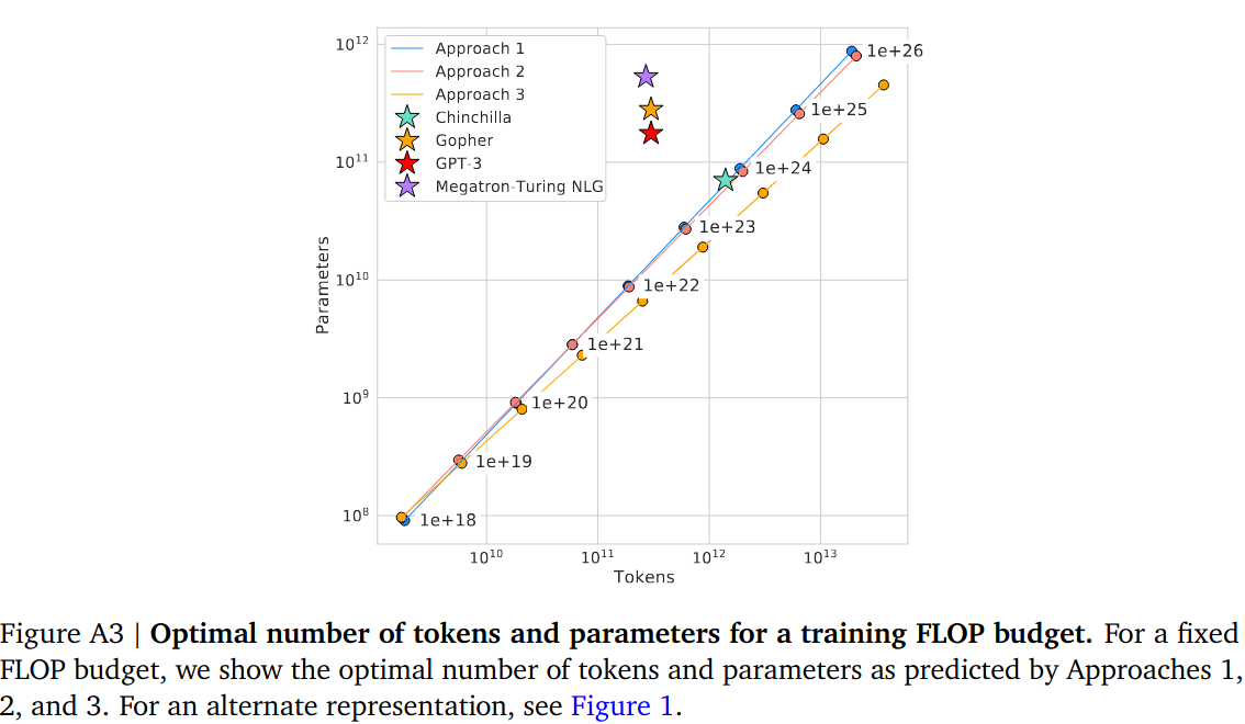
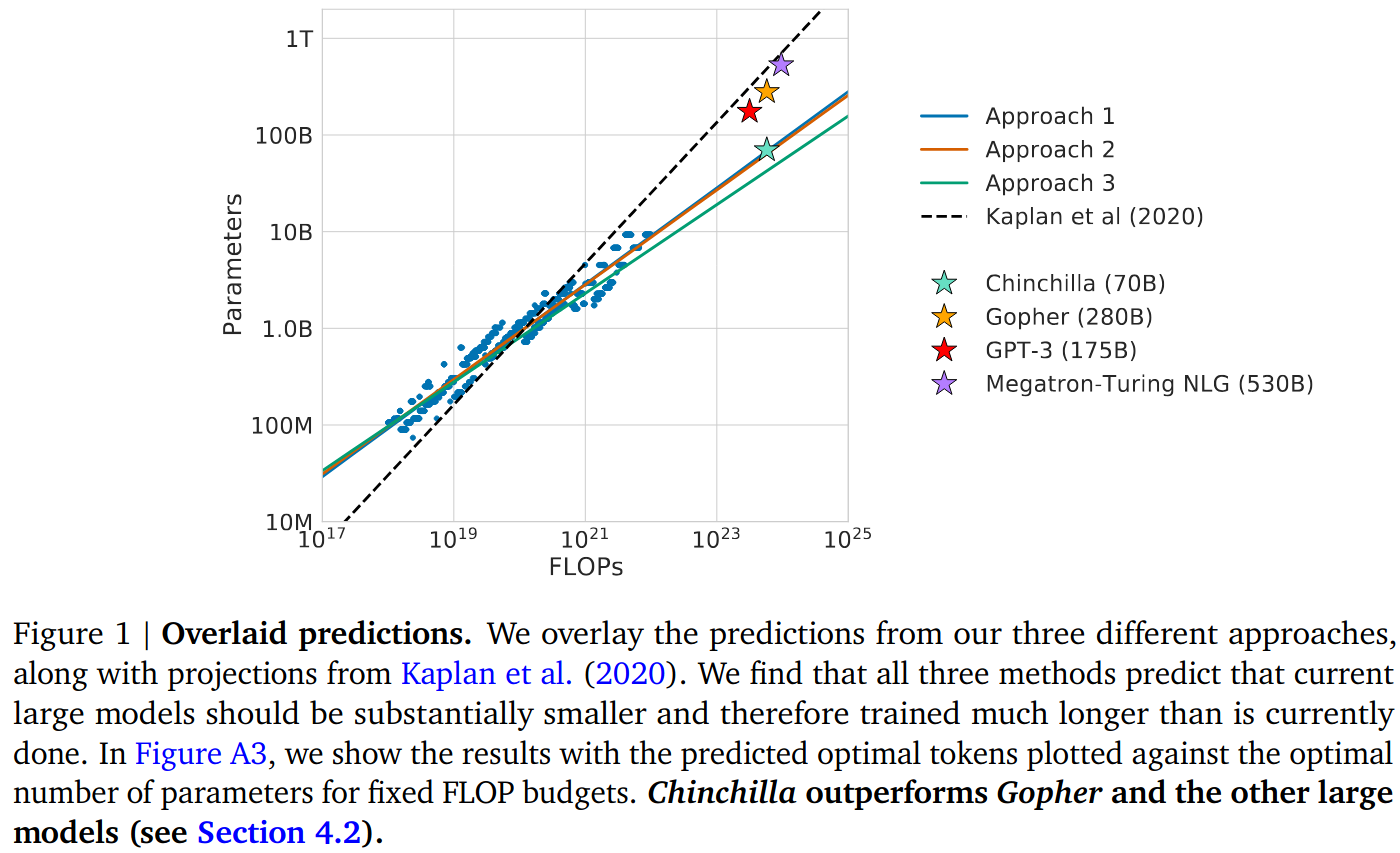
Figure 1 of the [2] is also interesting. It also includes Kaplan et. al line. Models trained until Chinchilla followed the Kaplan et. al scaling laws, and they seem to be undertrained. Training of Chinchilla validates Hoffmann scaling law and verifies that previous models were actually undertrained. This plot effectively summarizes importance of scaling laws.
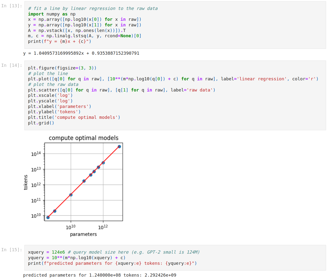
Andrej Karpathy published a brilliant notebook[4] that uses Table A3, Approach 2 data to fit a line and make projections. Following code from [4] shows the trend line.
Llama 3 Scaling Laws
In [3], llama-3 paper introduces its own scaling laws with similar assumptions. The power relationship between compute and dataset size is given in:
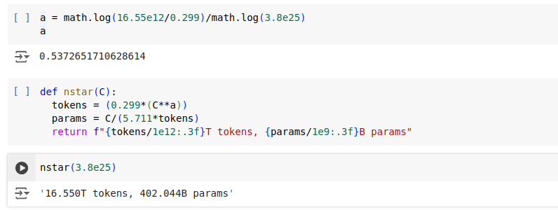
\[N^{*}(C) = AC^{\alpha}\]In the paper, \((\alpha, A)\) is given as (0.53, 0.29). Unfortunately, with these values it is not possible to recreate their projection of 402B parameters and 16.55T tokens.
Also they show deviation from FLOP approximation of Kaplan [1]. They seem to use a slightly different approximation:
\[C = 5.711 * N * D\]which can be easily found by using their compute budget, and projected parameter count and dataset size. From this point on, one can leave A as-is and try to obtain a better estimation of α .
\[N^{*}(C) = AC^{\alpha}\] \[16.55*10^{12} = 0.299*(3.8*10^{25})^{\alpha}\] \[16.55*10^{12} / 0.299 = (3.8*10^{25})^{\alpha}\] \[log(16.55*10^{12} / 0.299) = \alpha x log(3.8*10^{25})\] \[\alpha = 0.5372651710628614\]With this value, it is possible to match values in the paper:
Conclusion
Scaling laws is a great tool to plan ahead of pre-training. Scaling laws provides a loose estimate of optimal dataset size or model size. While scaling laws are important and widely respected, there are counter examples.
Llama 3 models [3], other than the flagship model, continued training and hugely exceeded optimal dataset size. The idea is that while training beyond the optimal dataset size produces diminishing returns at model quality, it is well worth to have an inference optimal model, especially when inference costs are expected to exceed training costs.
References
1- Scaling Laws for Neural Language Models