Demystifying Neural Network Activations In Pytorch

October 15, 2024 8 minute read

Backpropagation is a crucial part of the deep learning training process. It allows us to compute gradients and update our model parameters. This post is not about explaining how backpropagation works. There are many excellent resources online that explain backprop in depth. For a few recommended materials you mays see [1,2].

Training large neural networks requires a lot of GPU memory and activation memory is a significant contributor to the memory consumption.

In this post I will try to demystify the activation memory in neural networks. It is difficult to find good materials explaining the nature of activation memory. I hope this post will be useful.

This post assumes a basic understanding of how backpropagation works.

What is activation memory ?

Consider the following linear transformations which are very common in neural networks:

\[z = Wx\] \[y = z + b\]

The partial derivatives are:

\[\frac{\partial z}{\partial x} = W\] \[\frac{\partial z}{\partial W} = x\] \[\frac{\partial y}{\partial z} = 1\] \[\frac{\partial y}{\partial b} = 1\]

We need to find derivatives of y wrt. x and W, which gives how sensitive is y to the W and x. By chain rule:

\[\frac{\partial y}{\partial x} = \frac{\partial y}{\partial z} \cdot \frac{\partial z}{\partial x} = \frac{\partial y}{\partial z} \cdot W\] \[\frac{\partial y}{\partial W} = \frac{\partial y}{\partial z} \cdot \frac{\partial z}{\partial W} = \frac{\partial y}{\partial z} \cdot x\]

Note that we need derivative of y wrt. z to calculate partial derivatives. In this example they are obvious, but in a deep neural network it is usually not the case.

Here is a simple multiplication implementation for pytorch:

class Multplication(Function):
    @staticmethod
    def forward(ctx, W, x):
        ctx.save_for_backward(W, x)
        output = W*x
        return output

    @staticmethod
    def backward(ctx, grad_output):
        W, x = ctx.saved_tensors
        grad_W = grad_output * x
        grad_x = grad_output * W
        return grad_W, grad_x

Note the grad_output parameter. It is the gradient of the output generated in the forward pass. For our example, in math terms, it is:

\[\frac{\partial y}{\partial z}\]

This is the expression that we needed to calculate partial derivatives above. Now lets repeat what we have learnt: In order to calculate partial derivatives, we need the gradient of the output and some variables. Output gradient is provided by pytorch.

Since we need input variables in backward pass to calculate partial derivatives, we need to save them in forward pass. This is the source of activation memory.

In multiplication case, variables are operands, namely x and W. For other operations, variables vary. Which variables are necessary for gradient calculation depends on the operation. e.g. for derivative of sum operation no variable is needed because derivative of sum is just 1.

Pytorch Tensors

In pytorch everything is a tensor. From memory point of view, network weights, input or activations are all the same. They are tensors saved in the memory.

Input tensors, typically, are not modified. They are not adjusted to improve the network output. Hence input tensors do not require gradients. Weights do require gradients. If a weight does not collect gradients it is said to be frozen.

For activations, if one of the inputs to the operation requires gradient, then the resulting activation also requires gradients. As a result, activations almost always requires gradients to be calculated.

An input to an operation can be one of weight, input or activation e.g. result from another operation.

What happens when a weight is used in an operation? What will happen if the weight tensor needs to be saved for backward pass? Will it occupy additional memory space? The answer is no! Pytorch will create a new tensor but it will point to the same memory location of the original weight tensor, thus no additional memory will be used.

Torch CUDA Caching Allocator

Pytorch uses a sophisticated CUDA allocator to manage CUDA memory efficiently. The idea is that cudaMalloc and cudaFree operations takes significant amount of time and introduce synchronization between CPU and GPU. In order avoid cudaMalloc and cudaFree calls as much as possible, pytorch requests block of memory from CUDA and tries to reuse them during the lifetime of the program.

The allocator rounds up allocation requests to avoid oddly shaped allocations which are likely to cause fragmentation. In default mode, allocations are rounded up to multiple of 512 bytes.

For more information about the CUDA caching allocator, your may see [3].

Computation Graph

During forward pass, pytorch creates a computation graph to allow execution of backward pass. For each forward call, a node that includes call to backward function is added to the computation graph.

This computation graph is core to the Pytorch’s backpropagation implementation. Loss value is the root of the graph, network weights are leaves of the graph. Intermediate nodes correspond to backward pass functions that calculates output gradients.

Here is the corresponding computation graph for a linear transformation defined above. Green node represent the root (output tensor), blue nodes represent leaf nodes (weight tensors), orange nodes shows tensors saved for backward pass and gray nodes represents backward pass functions.

Note that x is not part of the graph since it does not require gradients.

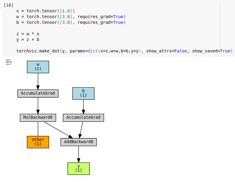
In the graph, you can see that multiplication operation saves w tensor for backward pass. Conversely, x is NOT saved, because it is not part of the graph. Also note that, Add operation does not save any tensors, because its derivative is 1 and does not depend on inputs.

You should also notice the AccumulateGrad nodes. These nodes are connected to the leaf nodes and used for accumulating gradients during backward pass.

In pytorch, there is a special layer for multiplication followed by an addition: nn.Linear. We can plugin nn.Linear layer to achieve them same output with less code.

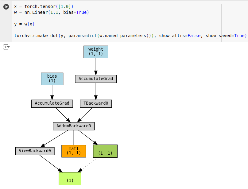
Note that instead of two functions, nn.Linear introduces single function: AddmmBakward0. Similarly, AddmmBakward0 caches only the weight tensor (mat1). Dark green node indicates that the output tensor (light green tensor) is a view of the output of the Addmm operation. Rest of the graph looks similar.

Automatic Mixed Precision Training (AMP)

Another interesting aspect to of the computation graphs would be to see how Automatic Mixed Precision Training (AMP) looks.

Neural network weights are stored as 4 byte floats. Float32 is called full precision. Modern GPUs performs matrix multiplication much faster at half precision, float16. However, half precision is not suitable for some operations. Using solely float16 significantly degrades training performance. AMP strikes a balance between full precision and half precision. In AMP, some operations use full precision while others use half precision.

Here is how the computation graph in mixed mode looks like. Note ToCopyBackward0 functions. They indicate that tensors are down scaled to half-precision.

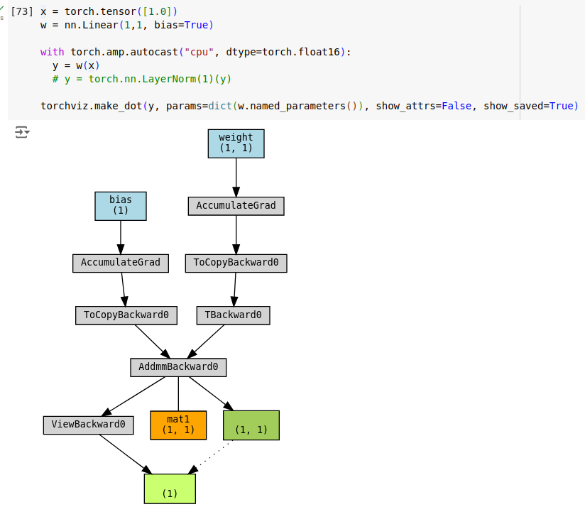
Unfortunately, torchviz does not display precision information. But we can obtain this information by traversing the computation graph. Here is a BFS code to traverse the graph and print function and tensor data.

from collections import deque
import torch

def is_tensor(t):
    return isinstance(t, torch.Tensor)

def shape(t:torch.Tensor):
    return list(t.size())

def bsf_print(y, named_parameters=None, print_saved_tensors=True):
    
    named_parameter_pairs = list(named_parameters)
    accounted_address= set()
    parameter_index = dict()

    if named_parameters:
        parameter_index = {tensor:name for name, tensor in named_parameter_pairs}
        accounted_address = { t.untyped_storage().data_ptr() for n,t in named_parameter_pairs}

    queue = deque([y.grad_fn])
    visited = set()
    
    print("")
    print("Computation graph nodes:")

    while queue:
        node = queue.popleft()
        if node in visited:
            continue

        visited.add(node)

        if "AccumulateGrad" in node.name():
            tensor_var = node.variable
            assert is_tensor(tensor_var)
            assert tensor_var.requires_grad
            
            # do not add this to activation calculations
            accounted_address.add(tensor_var.untyped_storage().data_ptr())

            if tensor_var in parameter_index:
                print(f"* AccumulateGrad - {parameter_index[tensor_var]} - {list(tensor_var.size())} - dtype: {str(tensor_var.dtype):8} - Addr: {tensor_var.untyped_storage().data_ptr():13}")
            else:
                print(f"* AccumulateGrad - 'Name not known' - {list(tensor_var.size())} - dtype: {str(tensor_var.dtype):8} - Addr: {tensor_var.untyped_storage().data_ptr():13}")
        else:
            print(f"- {node.name()}")
        
        saved_tensor_data = [(atr[7:], getattr(node, atr)) for atr in dir(node) if atr.startswith("_saved_")]
        if saved_tensor_data and (print_saved_tensors):
            tensor_data = [data for data in saved_tensor_data if is_tensor(data[1])]

            # handle tensors
            if tensor_data and print_saved_tensors:
                for data in tensor_data:
                    t = data[1]
                    print(f"[{data[0]:>13}] - dtype: {str(t.dtype)[6:]:8} - Shape: {str(shape(t)):<18} - Addr: {t.untyped_storage().data_ptr():13} - NBytes: {t.untyped_storage().nbytes():>12,} - Size: {t.dtype.itemsize*t.size().numel():>12,}")
        
        # add children to the queue
        queue.extend([next_fn_pair[0] for next_fn_pair in node.next_functions if next_fn_pair[0] is not None and next_fn_pair[0] not in visited])

Now print the graph of the y tensor.

bsf_print(y, named_parameters=w.named_parameters())

AccumulatedGrad nodes represents the weight tensors. Note that weights are in full precision. mat1 tensor saved by AddmmBackward0 function is half precision version of weight tensor of the linear layer. The same tensor is kept in full and half precision. Total memory consumption is higher than using only full precision.

Computation graph nodes:
- ViewBackward0
- AddmmBackward0
[         mat1] - dtype: float16  - Shape: [1, 1]             - Addr: 98196682887744 - NBytes:            2 - Size:            2
- ToCopyBackward0
- TBackward0
* AccumulateGrad - bias - [1] - dtype: torch.float32 - Addr: 98196682467904
- ToCopyBackward0
* AccumulateGrad - weight - [1, 1] - dtype: torch.float32 - Addr: 98196682648256

If you uncomment nn.LayerNorm line and view the tensors, you will see that LayerNorm is sensitive to precision thus keeps its values in full precision.

Activation Checkpointing (Gradient Checkpointing)

Activation Checkpointing (AC) is a strategy that trade offs activation memory usage and training speed. In activation checkpointing, intermediate activations are not stored. Instead intermediate activations are calculated again. This approach saves some space but introduces extra calculations.

Let’s revisit the linear layer example. This time input tensor is initialized to require gradients. Please note that intermediate activations typically requires gradients.

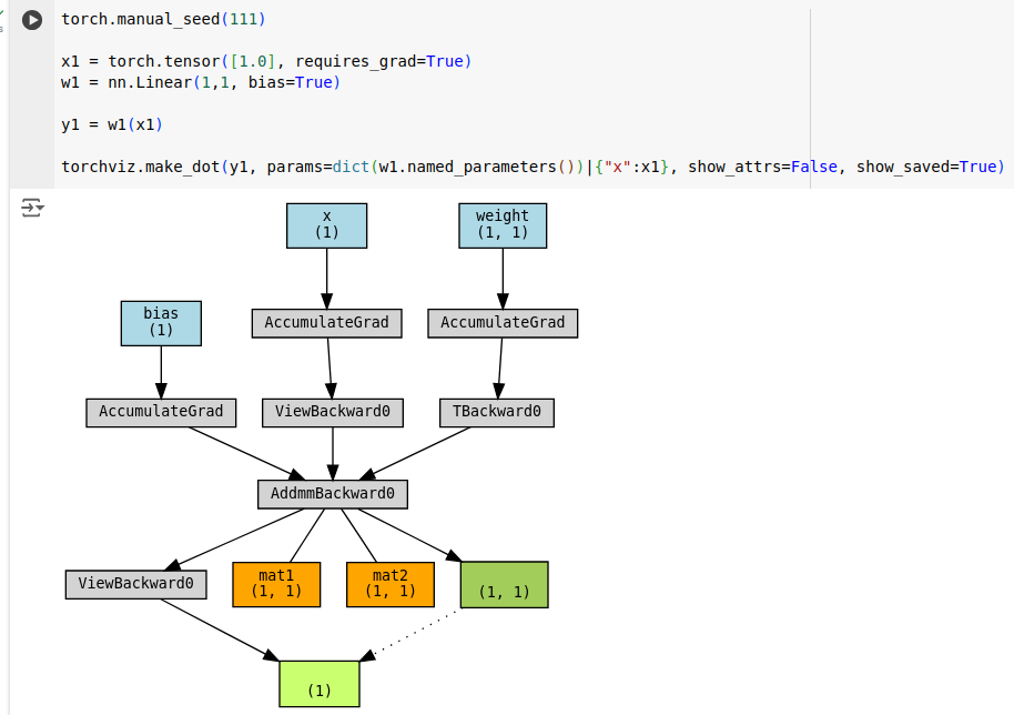
Now let’s enable gradient checkpointing.

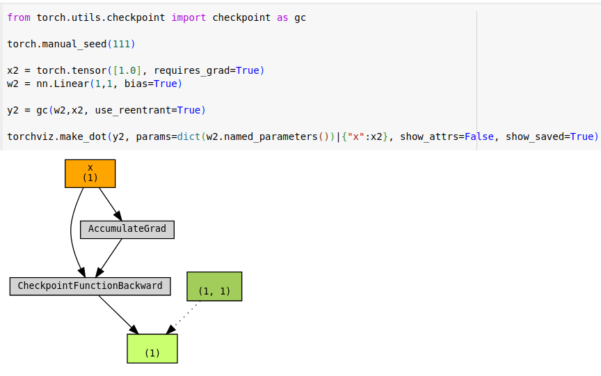
With AC, only the input tensor is cached. For larger networks savings will more prominent. Let’s verify AC does not break the original code.

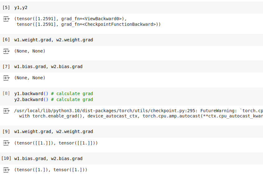
It is verified that outputs and gradients check out.

Conclusion

I tried to provide useful insights about understanding activation memory. Pytorch is a sophisticated library that does a lot of things to make deep learning fun for the developers. I really appreciate it. I would like to refer the reader to [7], excellent work of Andrej Karpathy, to see how would deep learning would like without libraries like pytorch.

For the notebook including the demo code, see [4].

For more detailed insight into transformer activation memory internals, see [5]

If you want to read more you may refer to [6] for a nice blog post about pytorch and activation memory.